Special thanks to Katelyn Chirdon for feedback and edits
Most online resources explaining Maxwell’s Equations are either written for university students recently trained in multivariable calculus, or are written for the general reader and avoid all discussion of math whatsoever. The relevant Wikipedia page is a good example of the first type, and this WIRED article is a good example of the second.
Both of these are good and valuable in the right contexts, but what I am after is something different. I want to understand how these equations are actually used, and for that, I do need to understand their mathematical forms. However, I am not interested in learning how to compute the equations myself; that is literally what the computer is for. What I need is just enough mathematics to allow me to gain a practical and intuitive understanding of Maxwell’s Equations, and that is what these notes seek to provide. As it turns out, this is significantly easier than learning enough mathematics to be able to compute the correct solution for complex problems. If you would like to learn how to do that, https://www.maxwells-equations.com/ is lovely
The following assumes that the reader has some familiarity with high-school algebra and electromagnetism. However, readers who are concerned that they do not have enough math or physics knowledge should continue reading regardless. I am writing this blog post precisely because I believe that you do not need to understand how to compute a triple integral or find the potential function of a vector field, in order to see the beauty of these equations or understand how other circuit laws may be derived from them.
In Part 1, we will describe calculus of a single variable. In Part 2, we will extend these ideas to multivariable and vector calculus, and in Part 3, we will examine Maxwell’s Equations with that vocabulary and toolset. Ready? Then let’s get started.
Let’s begin with some algebra. I have two unknown quantities, and I refer to them by x and y. I can write equations that describe the relationship between these two variables, such as y=3-x or y=x^2. These equations show how a change in x affects a change in y. When working with equations of two or three variables, we can often gain intuition about the behavior of equations by graphing them as below.
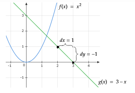
You may notice that this graph does not show y=x^2 and y=3-x, but f(x)=x^2 and g(x)=3-x. Here, we are defining the equations as functions, which is a relationship between two variables that has the additional property that every input has exactly one output. Graphically, this means that the curve is smooth (no holes/discontinuities, such as x=0 for y=1/x) and passes the ‘straight line test’ (a straight vertical line moved left to right along the entire graph of the function will only ever intersect the function once. An example of a graph that fails this test is a circle).
As you can see from the description above, both algebraic equations and geometric graphs are valuable ways to understand the behavior of functions. The algebraic approach is ideal for computing equations and proving theorems, while the geometric/graphical approach is ideal for quickly gaining overall intuitive familiarity. Thus, we will typically focus on the graphs of functions below, while also giving the precise algebraic equations for reference later.
In the graph above, we see that g(x) is a straight line. This means that its equation can be written in the form f(x)=mx+b, with m=-1 and b=3. m is called the slope of the line, and it is the rate of change of the single variable x. In this case, the slope is constant at -1.
f(x) is not a straight line, but we would still like to be able to use the notion of slope. For instance, g(x) could represent the position of an object moving at constant speed over time. The speed is equal to the rate of change of the function, which in this case is -1.
In this scenario, f(x) could represent the position of an object moving at constant acceleration, such as an object in freefall. We would like to be able to compute the rate of change of position of the object. Graphically, this would be equivalent to placing a line at every point whose slope is the rate of change at that point. These lines would then be called tangent to the function. In the graph below, the dotted orange line gives the tangent line at x=1.
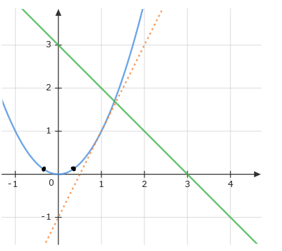
How can we find the slope of this tangent line? We can try to estimate it by plotting a line which intersects the graph twice, perhaps at x=1 and x=2. We can then calculate the “average slope” by dividing the change in y-value, Δy, by the change in x-value Δx. Then, by making Δx smaller and smaller, we obtain better and better approximations for the instantaneous rate of change at x=1:
| Point 1 | Point 2 | Δy | Δx | Δy/Δx |
| (1,1) | (2,4) | 1 | 3 | 3 |
| (1,1) | (1.5,2.25) | 1.25 | 0.5 | 2.5 |
| (1,1) | (1.1,1.21) | 0.21 | 0.1 | 2.1 |
| (1,1) | (1.01,1.0201) | .0201 | .01 | 2.01 |
If we instead wish to calculate the exact instantaneous rate of change for x=1, we will need a different tactic. Let us now consider the following limit –
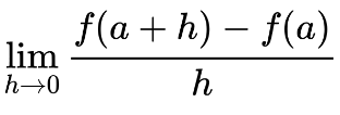
The expression inside the limit is just the formula for slope expressed in function notation. Change in x is represented by the distance h, and change in y is calculated as the difference between the value of the function at x=a and the value of the function at x=(a+h). Recall that our estimates of this value got better as h grew smaller. Hypothetically, if we could set h=0, then our “approximation” would perfectly align with the tangent line (why?). But division by 0 is a big mathematical no no, so there’s nothing we can do…or is there?
A limit is a way to express the behavior of a function around a given point, without expressing anything about the point. In the expression above, then, the limit does not represent the value of the expression at h=0, but instead at a point an infinitesimal distance away. An infinitesimal is a tiny number, smaller than any other number you can think of, and so the slope of the tangent line at x=1+h is just as good as the slope of the tangent line at x=1 for our purposes.*
We can go further, and calculate a new function that gives the slope for any value of a. This function is called a derivative, and the process of finding it is called differentiation. It can be written as f'(x), dy/dx, or d/dx[f(x)]. Graphically, it gives the slope of the tangent line to f(x) for any given x. In fact, slope is just the name we give to derivatives of functions of the form f(x)=mx+b.
Notice the similarities between the expression for a derivative, dy/dx, and a slope, Δy/Δx. It can be helpful to think of the second formula as the formula for average rate of change, and the first as the formula for instantaneous rate of change.
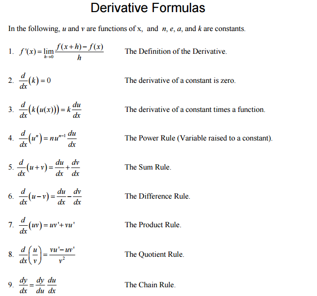
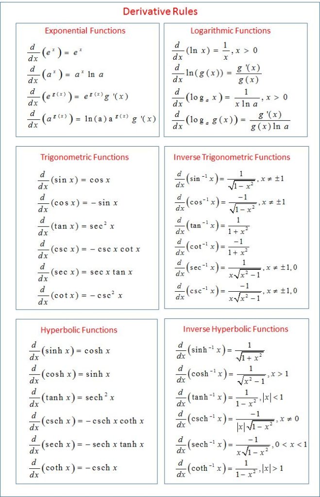
The following rules help to simplify the computation of complex derivatives:
* Infinitesimals are a great way to intuitively understand calculus. However, as it turns out, they are not mathematically rigorous, which is mathematician speak for ‘useless nonsense’. We know this because Isaac Newton and his mentor Edmund Halley got in a fight with Bishop Berkeley of the Anglican Church of Ireland, and Berkeley responded by disproving infinitesimal calculus. However, even after mathematicians confirmed that his reasoning was sound, people kept doing calculus, because it worked. In the 19th century they invented a dark art called ‘epsilonics’ to put calculus on a firm mathematically rigorous footing, so they wouldn’t have to feel weird about that. And then, in the 20th century, people decided even that wasn’t good enough, and so they invented a whole other system of numbers called the hyperreals which are designed specifically to invalidate Bishop Berkeley’s arguments and make infinitesimals mathematically rigorous.
What does all of this mean for us? Unless you’re in a place where you care about the mathematical rigor of your proofs, and you’ll know if you are, it doesn’t affect the calculations. So, compute away, and remember, every time you act as though infinitesimals were a valid concept for the real numbers, you poke Bishop Berkeley in the eye.
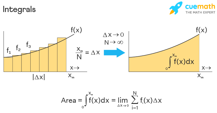
We can also use limits to calculate the area under a curve. We approximate the area with a series of rectangles, and use a limit to increase the number of rectangles to the point where we pretend each rectangle has practically zero width. It takes a lot more than that to first define and then compute these “integrals”, as the area under the curve is known. But, we don’t have to do that. Just look at this picture and bask in the glory of intuitive understanding without rigorous calculation –
Oh, btw, you know how addition and subtraction are inverses? Each cancels out what the other does, so (x+a)-a = x for all x and a that that question makes sense for. Similarly, multiplication and division are inverse operations, and a*(x/a)=x for all x and a. Wouldn’t it be convenient if we had inverse operations for differentiation and integration?
We do! It’s the Fundamental Theorem of Calculus! We will not prove this fact!

Look closely at what’s happening here. We have a function f(t), which has a derivative f'(t). The area between the x-axis and the graph f'(t), from point a to b on the x-axis, is equal to the difference of f(t) between just those two points. In other words, while complete knowledge of the values of f'(t) in the interval [a,b] is necessary to compute the left side of the equation, the right side only requires knowledge of f(t) at t=a and t=b. This is significantly easier to compute – but first requires us to find an f(t) such that d/dt[f(t)] = f'(t), and that is why integration is so much more difficult than differentiation.
That takes us through calculus of a single variable. This is about what you’d cover in a typical Calc I course, except that we don’t actually know how to solve any calculus problems. If you would like to learn to do so, one of many excellent free resources is MIT’s Single Variable Calculus course, available on their OpenCourseWare platform. In the next post in this series, we’ll extend these ideas to multivariable and vector calculus, and develop the notions of line integrals, surface integrals, curl, and div. After that, we’ll be ready to tackle Maxwell’s Equations, now equipped with an understanding of what all those little squiggles actually mean. Stay tuned!
Leave a Reply